Your data layer matters more than ever

Xarray Community Developer
We just built and released two new data exploration apps, OpenCell (details) and SanctSound (details).
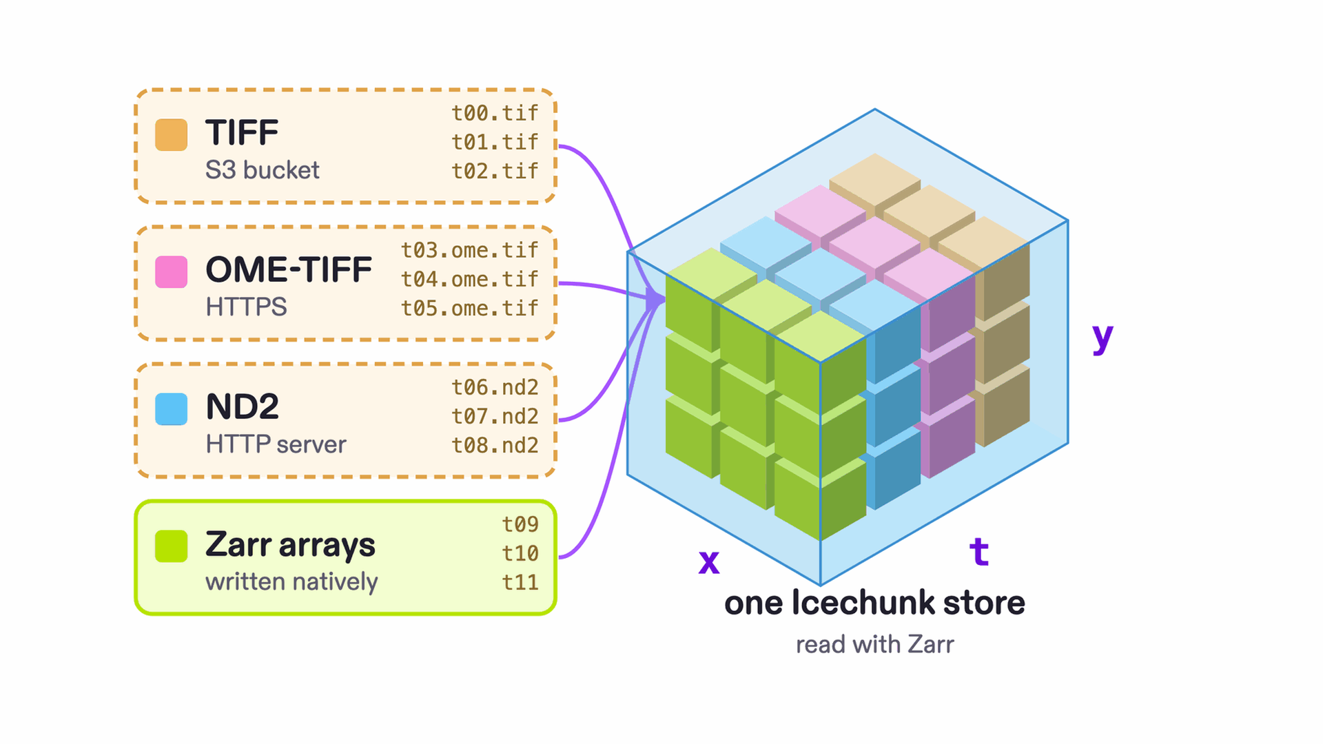
These were possible to develop quickly because the underlying datasets were zero-copy ingested into Icechunk. Zero-copy ingest presents the original files as one organized Zarr dataset without copying them. This meant we could devote all of our focus to building a great data exploration app, thinking about how to show the data and what the UI should be, rather than building data loading code and taking on its technical debt.
The data curation and organization being persisted in Icechunk means it’s easy to share. So anyone can access our organized version of the raw data which is freely available on Arraylake ( earthmover-biology/opencell, earthmover-biology/sanctsound).
1. Anyone can build a viewer now
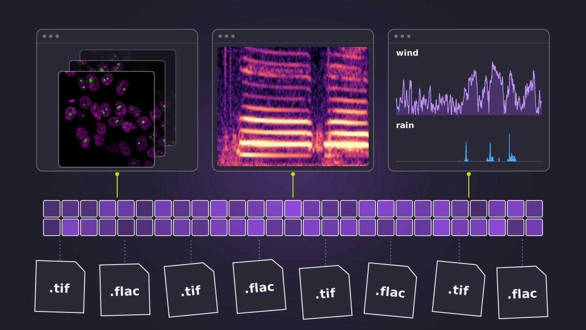
Today, with agentic coding, anyone can build a complex visualization or data exploration app in a day. This is possible to do by pointing an agent at the buckets of raw data. For our examples the raw data lives in OpenCell’s S3 bucket and NOAA’s SanctSound bucket on Google Cloud, which look like this:
s3://czb-opencell/microscopy/raw/
  AATF_ENSG00000275700/
    OC-FOV_AATF_ENSG00000275700_CID001083_FID00026474_proj.tif
    OC-FOV_AATF_ENSG00000275700_CID001083_FID00026474_stack.tif
    OC-FOV_AATF_ENSG00000275700_CID001083_FID00026475_proj.tif
    OC-FOV_AATF_ENSG00000275700_CID001083_FID00026475_stack.tif
    …
  …
gs://noaa-passive-bioacoustic/sanctsound/
  audio/ci01/sanctsound_ci01_01/audio/
    SanctSound_CI01_01_671379494_20181031T220000Z.flac
    SanctSound_CI01_01_671379494_20181031T235954Z.flac
    SanctSound_CI01_01_671379494_20181101T025952Z.flac
    …
  …
Pointed directly at those buckets the agent would engineer some bespoke data loading code, and maybe some sidecar files to record how the various raw files relate to each other.
But doing this costs time, tokens, compute, and the most precious resource, human attention. All of those resources spent on data wrangling could have been much better spent on building the data app itself. Furthermore, the resulting system is more fragile and less shareable than encoding the structure of the dataset into Icechunk.
In Icechunk, the same two datasets look like this:
group/ · array
earthmover-biology/opencell
  plates/               176 OME-Zarr HCS plates
    PML0264/E/9/        plate/row/column: well E9
      FID00026474/      a field of view, gene AATF
        0               (c, z, y, x) 2 × 106 × 600 × 600
        proj/
          0             (c, y, x) 2 × 600 × 600
      FID00026475/
      …
  projections/
  unlisted/             86 more cell lines
earthmover-biology/sanctsound
  CI01_01/              one deployment
    audio/
      waveform          367,183,364,448 samples
      segments/         355 recordings
        start_time
        end_time
        start_sample
        …
    detections/         2,008 events
    sound_levels/
    temperature/
    calibration/
  CI01_02/
  …                     8 deployments
2. Determining dataset structure is expensive - share it
A dataset is more than just the values in the arrays. A complete definition includes metadata, layout of the different arrays and how they relate to each other. Having a clear and self-describing dataset is a prerequisite to enabling people and their agents to explore and interact with the data.
Figuring out how to correctly assemble many raw files into a single related dataset needs skill, time, and thought. In all but the simplest cases doing it well requires human effort. So in the age of agentic coding, sharing the results of determining the structure of a dataset is more important than ever.
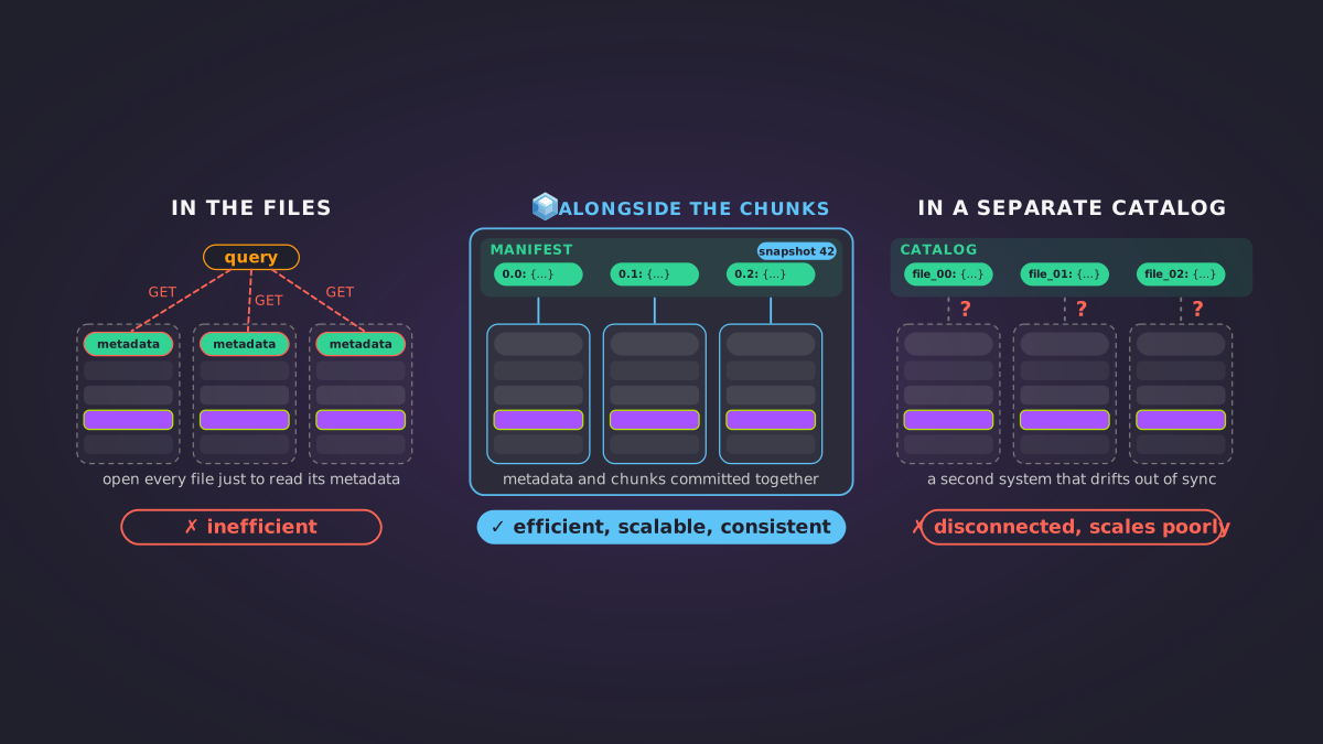
A common solution to this problem is to encode our knowledge of the dataset’s metadata and layout in software, i.e. with a specialized loader library. This is a valid and viable strategy, but encoding it into the format instead is more robust, transferable and immediately works in many programming languages. A loader library requires maintenance, may need to be rewritten for multiple programming languages, and most importantly does not travel with the data. So if someone finds the data, but not the library they will have to duplicate your efforts.
In contrast, encoding our knowledge of a dataset into the data format itself means that anyone who discovers your data can read it, not just anyone who discovers the data, and then also happens to find your library to be able to interact with it.
For an in-depth discussion of why metadata traveling with the data in the way Icechunk allows you to is important read our recent post How to make scientific data archives AI-ready. The core points that are relevant here are:
- Scientists care about datasets, not files.
- Metadata inside files can’t guarantee consistency.
- Humans and agents need the same things from storage.
Despite all these advantages of a self-describing dataset, a common reason people do not do it is that converting to Zarr means copying the data, and no one wants to delete their raw files, so the storage doubles. That is ok for a few GB, but for these datasets (OpenCell’s raw images are 912 GB, and NOAA’s SanctSound bucket holds 50 TB) duplicating the storage is unacceptably costly. Zero-copy ingest removes that cost: Icechunk stores references to byte ranges in the original files, so the raw files stay where they are and readers see ordinary Zarr. For the full explanation, read Fundamentals: What is zero-copy ingest?.
Working with data in Icechunk also gives you and your agents a much more robust, easy to work with, and safe storage primitive. Icechunk versions your data like git, with commits and rollback. That matters for datasets with regular updates and for reproducibility, and even for archival datasets like these two, whose metadata and layout we can keep improving as we find problems. Readers always see a consistent view, even while new data is being written, so an app or an agent never reads a half-finished update. (More in Versioning and integrity.)
3. The applications
These concepts apply across many domains of science. For our first two data exploration applications we chose a cell biology microscopy dataset and a marine bioacoustics dataset.
OpenCell
What it shows
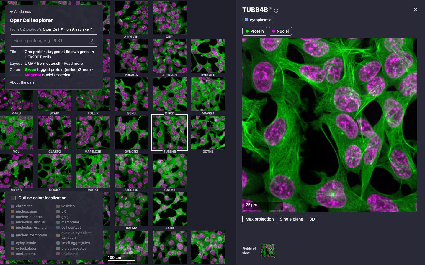
OpenCell is a CZ Biohub project that tagged human proteins with a fluorescent marker, one protein per cell line, and imaged the living cells under a microscope. Each image shows the cells’ nuclei in magenta, and the localization of the tagged protein in green.
In the explorer, the images are laid out one tile per protein arranged by UMAP according to their cytoself embeddings. This means that proteins that localize similarly to each other are near each other in the map. If you zoom all the way in to a tile or click on it you can explore the z-stack in 3D and see other fields of view.
Determining the structure
Dataset ingestion decisions, now encoded in the store:
- Plate layout. The bucket has one folder per gene. We regrouped the images into OME-Zarr HCS plates, with each max projection inside its stack.
- Metadata from OpenCell’s API. Each file name carries a cell line and field-of-view ID, which we used to attach the API’s record to each image.
- Imaging plates. The API lists two plates per image: where the cell line was made and where it was imaged. We used the second.
- Channel names. The TIFFs don’t name their channels, so we labeled them (nuclei, then the tagged protein) from OpenCell’s description of the dataset.
- Pixel size. The TIFFs say 0.2 µm, but the 63× objective and 13 µm camera pixels described in the OpenCell paper work out to 0.2063 µm. We use the optics value and keep the TIFFs’ beside it.
- Gene IDs. For 37 cell lines the Ensembl ID in the bucket path differs from the API’s. We store both.
- Unlisted cell lines. 86 cell lines are in the bucket but not on OpenCell’s website. They have their own
unlisted/group.
SanctSound
What it shows
SanctSound is a NOAA and US Navy project that recorded underwater sound in US marine sanctuaries from 2018 to 2022. Its underwater microphones (hydrophones) picked up whales and fish, wind and waves, and ships.
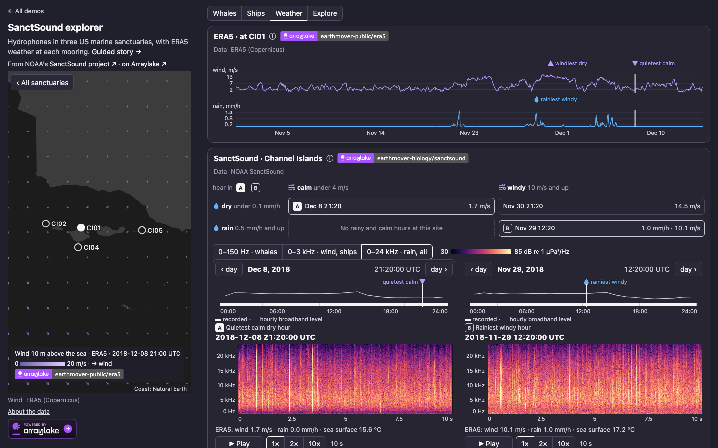
The explorer puts three of those sanctuaries on a map, where you can play each recording and watch its spectrogram. The Weather tab adds ERA5 wind and rain at each mooring, so you can find the calmest and stormiest hours and compare how they sound.
Determining the structure
Dataset ingestion decisions, with no community standard to follow:
- Recording layout. The bucket has one FLAC file per recording, 355 for a single deployment. We joined each deployment’s recordings into one continuous audio array.
- Timestamps. Recordings overlap and have gaps, so a sample’s position doesn’t give its time. A
segmentstable records when each recording starts, and the store’s metadata says how to use it. - Irregular chunks. FLAC frames don’t fall on a regular grid, so the audio uses Zarr’s variable-size (rectilinear) chunks.
- Detection events. NOAA’s detection files for whales, fish, ships and sonar use different time formats, and most have a
timevariable that is all zeros. We combined them into one table of events with real start and end times. - Small products. The hourly sound-level products are small, so we copied them into Icechunk with better chunking. Only the audio is virtual.
- Source metadata. NOAA’s DOI, license, citation and instrument details are spread across the product files and sidecar documents, not stored with the audio. We attached them to each deployment, along with its location, depth and time coverage.
Combining with ERA5
The explorer reads two Icechunk stores in the browser, earthmover-biology/sanctsound (virtual chunks in NOAA’s FLAC files) and earthmover-public/era5 (native chunks), and puts ERA5’s wind, rain and sea temperature on the same time axis as the audio. The two datasets come from different fields and different file formats, and the app reads both the same way.
4. Try it
Try out these datasets, earthmover-biology/opencell and earthmover-biology/sanctsound, or anything on the Earthmover Marketplace, and let us know what you make with them!
Xarray Community Developer