Plotting NYC heatwaves during NYC Climate Week

Calculating climate risk metrics from ERA5 using Arraylake, Icechunk, and Xarray.

Just show me the notebook!

Intro

This year at NYC climate week it’s been pretty hot and humid outside. This felt ironically appropriate while we ran a participatory workshop “Open Data in Applied Risk Analysis”, organised by GeoSpatial Risk and sponsored by Earthmover, showing how anyone can use public weather reanalysis data on the Earthmover platform along with some cool open-source tools to calculate the historical frequency of heatwaves over NYC. Let’s start with some cloud-native geospatial data.

Public ERA5 in Arraylake

ERA5 is a comprehensive global atmospheric reanalysis dataset produced by the European Centre for Medium-Range Weather Forecasts (ECMWF). Recently we added a copy of ERA5 in the Earthmover platform. The full ERA5 archive contains several petabytes of data, and whilst Zarr can reach that scale, this public Arraylake repo currently contains a 40TB subset of ERA5 - surface data with hourly global coverage back to 1975, and ~30km spatial resolution, up until Dec 31 2024.

Anyone can make a free Arraylake account and read this data. Try it! This shows how Earthmover customers can use the platform to provide easy public access to even very large datasets.

Finding historical NYC heatwaves using MetPy and XClim

For the workshop we showed a room of people how to calculate the number of days per year considered part of a heatwave in NYC, for every year going back to 1975. The actual calculation involves first computing the heat index using the National Weather Services’s definition (shown in a table below). For this we use some convenient functions supplied by the community-maintained MetPy package.

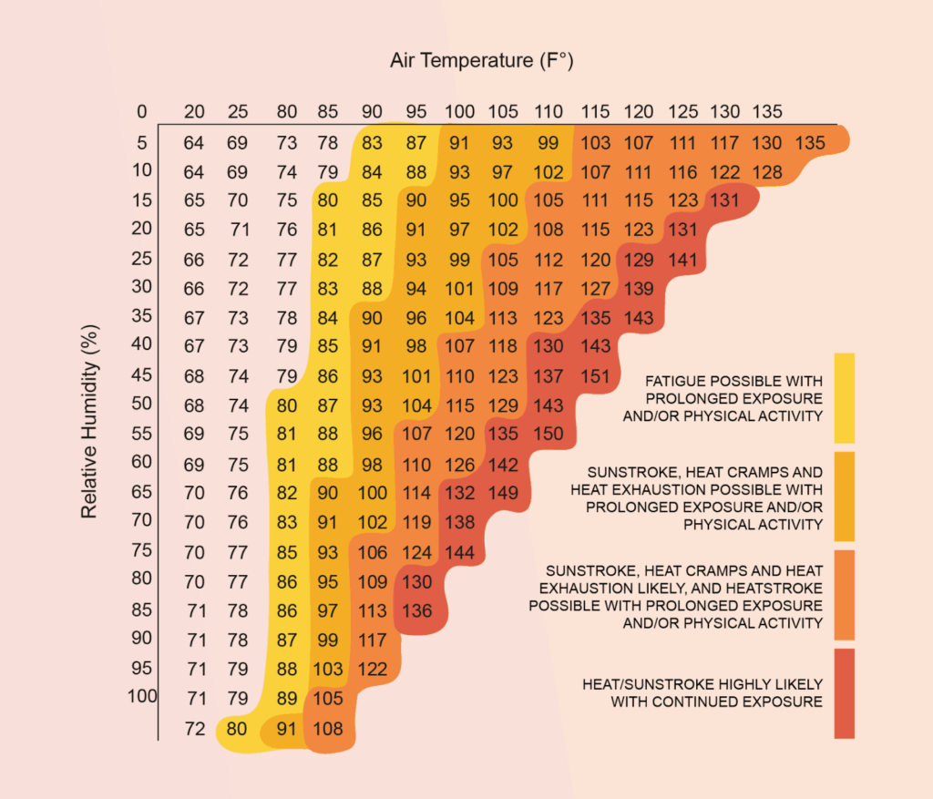
Table of the heat index as a function of temperature and humidity, as defined by the National Weather Service, and used by NYC authorities. (Source: National Weather Service via https://nychazardmitigation.com/)

Then we apply NYC’s local criterion for issuing a “heat advisory” - that the temperature be above 95F for 2 or more consecutive days. For this there is another convenient function we can use, this time from the XClim package.

The full calculation is in the notebook, but at the end we get a plot that shows the number of days per day for which a NYC heat advisory would have been issued. While we glossed over a couple of subtleties for this quick demo, the result appears basically consistent with the official NPCC report covering 1981-2017, which says NYC averages 17 days per year with maximum temperatures at or above 90°F and has heat waves lasting an average of four days. (The biggest difference between our analysis and the official report is that we used global reanalysis data whereas the official report used local meteorology station data, with different stations in different regions of the city.)

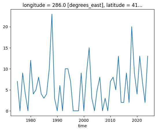
The number of days per year whose maximum heat index exceeded the threshold for issuing a heat advisory in New York City.

This is kind of wild. Using the public data, these open source tools, and Earthmover, in a few lines of python we already got close to the official weather record and hazard recommendations. This is an example of how cloud-native tools enable a huge democratization of what was once the province of elite scientists with access to supercomputers.

Even from a laptop this works so smoothly because:

Icechunk and Zarr efficiently fetch only the chunks required,
The original data is available with time-aligned chunking,
Xarray and Dask allow expressing the query in readable code, and lazily evaluating it.

This is an example of timeseries analysis at an arbitrary point on the globe, using custom functions. If you want to calculate climate or weather-related risks at particular spatial locations from forecast data it can be done in a very similar way. Note that these same packages also contain functions for calculating agricultural climate risk metrics, such as growing degree days.

Heat stress during the 2024 India heatwave

As a bonus exercise at the workshop, we also demonstrated some spatial analysis of the ERA5 data, this time plotting a map of heat stress during the height of the 2024 India heatwave.

This is pretty straightforward - we use the spatially-chunked version of the dataset, subset to a bounding box over India on an afternoon during its peak, then calculate a quantity called the wet bulb temperature (again using MetPy), which is a measure of heat stress on a human body.

Given that a wet bulb temperature of >95F is likely to be fatal even to fit and healthy people, the plot we obtain of its value over India and Bangladesh is pretty sobering - it means millions of people experienced weather worryingly close to being so hot and humid that you physically cannot sweat enough to stay alive outside.

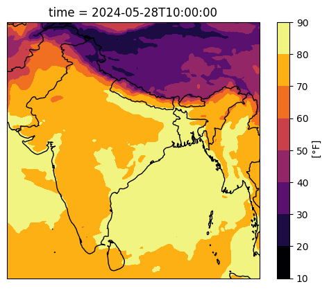
Plot of the wet-bulb temperature over India and Bangladesh during the 2024 Indian heatwave, calculated directly from ERA5 surface reanalysis data.

Tracking physical units with Pint

One detail in the notebook you might notice is that throughout these calculations we basically ignored the issue of ensuring that we were using the correct physical units (e.g. Fahrenheit vs Centigrade). That’s possible because we used the Pint package (and the bridge package pint-xarray) to handle these unit conversions for us!

Pint promotes raw numbers to “Quantities”, which attach a physical unit (such as Fahrenheit) to the data type. By automatically checking units and converting quantities during arithmetic, pint can detect or avoid types of errors which are otherwise impossible to identify. MetPy in particular has extensive support for pint, making it effortless to avoid bugs with imperial vs metric quantities. To learn more about how pint works with xarray read this blog post on pint-xarray that I wrote back in 2022!

Effortless reproducibility via marimo and uv

The final neat thing we used in this workshop was the combination of Marimo notebooks and the uv package manager. Using both these tools it’s just a one-liner to reproduce this notebook and its results on another machine.

The marimo notebook is saved as an executable python script (rather than as an `.ipynb` file, also available here), with the exact dependencies declared inline using PEP 732, which uv can understand. The result is that all our workshop attendees need only install uv (which takes one line) and then execute one line in their terminal to immediately get set up and start running code! If you’ve ever participated in a hands-on coding workshop where you spent half the workshop time getting set up, you’ll understand how awesome it is that this just works.

Conclusion

We did some spatial and temporal analysis of ERA5, from a laptop, calculated local climate metrics, utilising the power of both the Earthmover platform and the thriving open-source ecosystem around xarray.
If you want to use the Earthmover platform within your organisation then get in touch!