Having it all: virtual and materialized data products

dynamical.org

dynamical.org
We want it all:
- low-latency updates
- completeness over time, variables, and vertical dimensions
- access speed for time-series and map-style reads
But when your data is 14 PB and 1 billion GRIB messages, making that dream a reality takes some work. Virtual Icechunk Zarrs are a key complement to our materialized (rechunked) Zarrs. Together they get us one step closer to the catalog of our dreams.
We recently made a big push to build up our virtual Icechunk capabilities. This note describes why we create them, how we do it, and the lessons we’ve learned along the way.
Why go virtual?
For gridded weather data, thoughtfully designed virtual Zarrs offer three main benefits.
- Update latency. Because there’s no heavyweight data to move around, our stores can reflect new data within seconds of it becoming available at the source.
- Completeness across variables and vertical dimensions. In cases where native files are already available publicly, we avoid storing the data ourselves, letting us offer all variables at all vertical levels for more models, more quickly.
- Fast access. Native files tend to be structured in a way that’s optimal for reading the model’s entire geographic area at a single time step.
Adding virtual Zarrs gives us a catalog of options tuned to different jobs: our materialized (rechunked) products for training a regional time-series model across a forecast archive, our virtual products for low-latency inference, an analysis product as a proxy for observations, and so on.
Virtual what?
The geospatial data sector spends a lot of time optimizing, sometimes prematurely. Is this one of those moments? We think it isn’t: we started with the problems (latency, completeness) and worked backward, exhausting our existing techniques before picking up a virtual approach.
“Virtual Zarr?” you may be saying, “sounds like a Zuckerberg fever dream.” Nay, I say: a virtual Zarr is nothing more than a Zarr whose chunks are references to data stored somewhere else.
Every chunk in a virtual Zarr is backed by a virtual reference, and the reference is just a URL saying where to find the file, and the byte offset range to read within the file. The Zarr’s metadata also stores which codec to use to decode the bytes (netCDF, HDF5, GRIB2, etc.). If you are familiar with GRIB indexes, imagine someone combined every GRIB index from your favorite weather model into one gigantic index.
The virtual Zarr concept grew out of the challenge: “We have these huge piles of data in legacy file formats. We’d like to use it as an analysis-ready, cloud-optimized data cube, but we don’t want to reprocess and double-store all the data.” The kerchunk project pioneered this concept with the realization that by storing references that point to those legacy files, client libraries could read them on the fly, and the whole experience would act like a modern data cube. The VirtualiZarr project built on this, improving the ergonomics of constructing a virtual Zarr. Virtual capabilities were a natural addition to Icechunk. After all, references to chunks of data are core to how Icechunk achieves atomic updates and data versioning for virtual and materialized Zarrs alike.
There and back again: a virtual read
So what happens when you read ds["temperature_2m"].sel(time="…") from a virtual Zarr?
- Xarray translates your coordinate selection into integer indexes.
- Zarr finds which chunks those indexes fall within (e.g.,
temperature_2m/c/0/1/2andtemperature_2m/c/3/4/5) and asks the Zarr store for those chunks.
Up to this point, virtual and materialized Zarrs follow the same path. Here’s where they diverge:
- Because this store is virtual, Icechunk takes a chunk key like
temperature_2m/c/0/1/2and looks it up in its manifest to find a source URL and byte range, then fetches those bytes (from local disk, object storage, wherever the URL points). - Zarr picks back up, decoding the bytes using the
codecnamed in the Zarr’s metadata. In a materialized Zarr, that codec is often a standard compressor like zstd. In a virtual Zarr, it’s a codec that knows how to read the native file format: netCDF, HDF5, or for GRIB weather data, theGribberishCodec.
Once the bytes are decoded into an array, everything is back to standard Zarr: the array is indexed as usual, returning the values you asked for.
Virtual or materialized: which to use?
The short answer: try both, and see which is fastest for each of your access patterns. Within the same project it may be optimal to use both together.
For dynamical.org’s catalog, here’s a rule of thumb:
Does an individual unit of work read the model’s whole geographic domain? If yes, use virtual, else use materialized.
If a variable you need is only available in the virtual Zarr, try that and let us know at feedback@dynamical.org if the performance isn’t what you need. We add variables to our materialized Zarrs based on demand.
More generally, use the product that will fetch the fewest chunks of data for your access patterns. You can find the chunking of our datasets in the Earthmover Marketplace listings.
There’s nothing about virtual Zarrs that requires them to be faster for single-time-step, map, or spatial access patterns; it just happens that almost all native gridded weather data files follow that shape thanks to the mechanics of running a weather model. If someday we find native, time-series-optimized files, we’ll virtualize those and have our materialized dataset rechunk to optimize for spatial access.
How fast is fast?
Enough talk. Let us show you the numbers.
We define latency as the time between the moment a file first becomes available at the source and the moment that data is first available in our Zarrs — specifically, from a file’s “modified” or “created” timestamp at the source to the timestamp of the first Icechunk snapshot containing the same data.
These statistics are calculated on a relatively short history of our first virtual Zarr, NOAA HRRR forecast, 48 hour, virtual. As we build up a longer track record, we’ll add them to our data product pipeline status page, where you can audit the details and see them covered under tight latency thresholds in our SLA.
Latency (seconds)
| p50 | p95 | p99 | max | |
|---|---|---|---|---|
| all | 2.9 | 4.2 | 5.9 | 7.7 |
| surface | 3.2 | 4.5 | 5.8 | 6.0 |
| pressure | 3.1 | 4.2 | 6.1 | 7.7 |
| model | 1.7 | 3.7 | 4.7 | 5.9 |
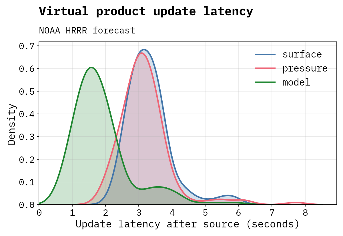
wrfnat) feed the fewest arrays and have the lowest latency, hinting there's even more room to optimize the larger surface and pressure groups.How we update them fast
Three priorities guided the design of our virtual Zarr update pipeline: fast, correct, resilient.
Push or poll? This is one of the core questions when designing a system that reacts to new data as it arrives. “Get notified right away” makes push notifications sound like the obvious choice wherever they’re available. As you get into the details, the story becomes more complex: a dataset that produces many files at once (e.g., an ensemble run) needs debouncing regardless, since committing takes about a second and many files can land in that same second. And most national NWP agencies’ operational file servers, the sources with the lowest latency, don’t support push notifications at all. Backfills would need their own handling too, since there’s no “new file” event to subscribe to for data that already exists.
Polling at a high rate (a second or less) collapses all of these cases into a single path. A backfill polls once, stores what’s there, and moves on; an update keeps polling until the full forecast has arrived. The same loop works across HTTP, FTP, and object stores, and across backfills and updates alike, eliminating a whole class of “two code paths drifted apart” bugs. It’s also resilient: if the process restarts, it catches back up on the next request.
An update in our code follows these steps:
- List all the files we expect to have when an update is complete. A quick, deterministic enumeration driven by the Zarr’s coordinate labels.
- Filter out the files we already have in our store. This is a fast existence check against the Icechunk manifest, not many network requests.
- Loop: ask the source if any of the remaining files are present. If they are, commit their virtual references to the store. Continue looping until the forecast is complete or you exceed a generous deadline to account for late forecasts.
If you’d like to get even more into the implementation, this is all in our open-source code.
Lessons
In the end, the bottlenecks to low-latency updates come down to:
- CPU: zstd decompression and compression of all the Icechunk manifests changed in a commit.
- Network: download/upload of all Icechunk manifests changed in a commit.
Even for large ensemble forecasts, an incremental update with well-tuned manifest splits (see below) can do this work in a couple of seconds on modest hardware.
That’s not to say it was fast on the first try. Lots of N² or serial loops that don’t matter at small N rear their heads at the scale of a billion references and over 100 Zarr arrays. But the good news is that they’re all solvable: (1) ultimately this is small data per update and computers are fast, and (2) AI does great with a verifiable objective, and wall-clock time is exactly that. We’re having fun working with AI to optimize this one.
Here’s an incomplete list of bumps we had to work out:
- Manifest splitting: just like optimal Zarr design depends on thinking through access patterns and sizing chunks accordingly, chunking the metadata is crucial in virtual datasets of substantial size. Too big, and commits are slow. Too small, and many tiny manifest files slow reads. Icechunk docs. Thanks to Tom Nicholas of Earthmover, who helped us think through manifest splitting. Check out his write-up on the history of GRIBs and virtualizing them.
- Manifest flush concurrency on commit: we contributed an optimization to Icechunk to let users configure the concurrency used when downloading and uploading changed manifests during a commit. This doesn’t need tuning unless you have lots of arrays being updated in one commit, but without it our end-to-end latency couldn’t have gone below 50 seconds. Thanks to Sebastián Galkin of Earthmover, this will probably be on Icechunk
mainby the time you read this. - Kubernetes node consolidation: just say no. Thirty-second container startup after moving your pod?! Gasp. Kubernetes trying to save us money isn’t something we want when we’re sensitive to seconds.
Data product design and usability
It’s not enough to make them fast; we also wanted these virtual Zarrs to be as simple to use as the rest of our catalog. Much of that happens for free by virtue of them being an Icechunk Zarr: Icechunk exposes a nearly uniform interface regardless of how the dataset is constructed.
A key element of ease of use for us was drop-in compatibility with our existing materialized Zarrs. For any variable in our materialized data products you can grab the same variable from the virtual product and you’ll get the same values out. To make this happen we apply a few select, on-the-fly transformations to make the values you get back from our virtual Zarrs exactly match those from our materialized Zarrs. Matt Iannucci, the creator of Gribberish (also working at Earthmover), has been very helpful along the way as we contributed a couple new GribberishCodec options that do those on the fly.
What’s the catch?
There’s a limit to how we can manipulate data to improve UX (although we do this sparingly). The two most salient: you won’t find a deaccumulated precipitation rate like in our materialized datasets, and we can’t homogenize a variable that switched units sometime in its history (e.g., hPa to Pa back in 2019).
What’s next
- For dynamical.org, we’ll create both virtual and materialized products for all popular datasets. You’ll find us initially releasing more virtual datasets since the commitment in ongoing storage is much lower.
- Virtual
grib2.bz2? (e.g., NOAA MRMS, DWD ICON-EU) You bet, thanks to the power of Zarr codec pipelines. - We’ll start virtualizing datasets that don’t have public data, e.g., ECMWF pre-schedule delivery. That will come with its own challenges (no GRIB indexes). Because there’s no need to decompress and recompress data, virtuals will still give us near-optimal latency.
- More optimizations: what we have works great for 175 variables, but what about a 400-variable dataset? (HRDPS anyone?) Good thing there’s more juice to squeeze.
dynamical.org
dynamical.org