Making open-source AI weather forecasting models easy to run

Emma Scharfmann

ML for Science
Hugging Face

Aaron Spring

ML, AI and geospatial data engineering

Ryan Abernathey

CEO Earthmover

Kashif Rasul

AI Research Science
Hugging Face

AI weather forecasting models now complement physics-based models while running far faster and on a fraction of the resources. Many of these state-of-the-art models are also open-weights: ECMWF’s AIFS models and Microsoft’s Aurora publish their weights directly on Hugging Face, and Google DeepMind has open-sourced WeatherNext 2. But open weights don’t make a model easy to run.

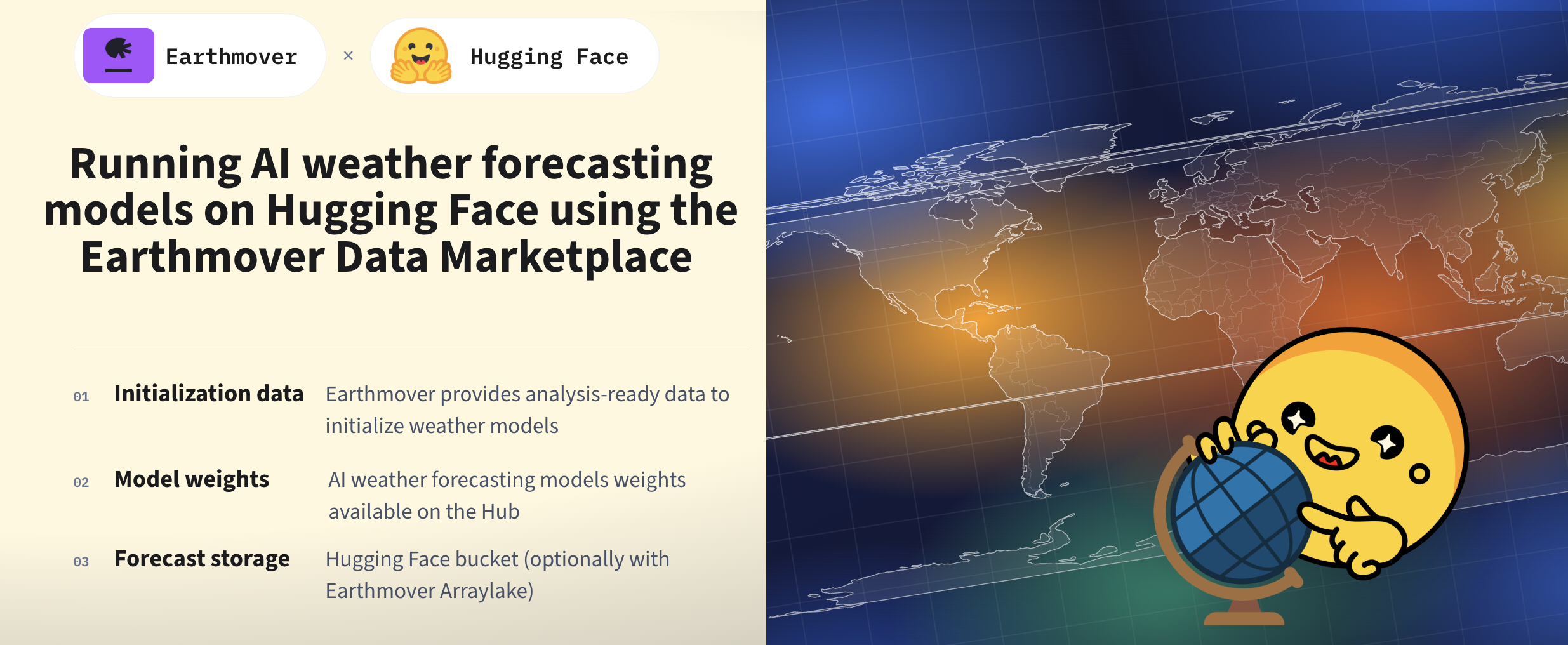
This blog post was written jointly by Earthmover and Hugging Face, and aims to reduce the friction of running open weather forecast models, using analysis-ready weather and climate data for initial conditions and validation. We’ll show you how to run different AI weather models on Hugging Face, and what data and data format can be used to run these models easily.

1. Why are we writing this blog post?
2. Running weather forecasting models yourself on our demo space
3. Tutorial: running an AI weather forecasting model locally with data from the Earthmover Marketplace
4. Earthmover: the Science Data Cloud
5. What’s next on AI for climate at Hugging Face?

Why are we writing this blog post?

In principle, AI weather models are lightweight enough to run on a laptop or a small cluster, as inference only takes seconds. With the right pipeline and tools, you should be able to run forecasts from any initial conditions, and evaluate them against historical climate data, without the need for large compute or storage. But, you will often run into some friction before reaching the inference step:

• Compute: Many models, including AIFS, depend on flash attention, which only works on certain GPU architectures.
• Storage: Downloading the data for one forecast is doable, but it doesn’t scale to real evaluation or training. Backtesting a model over a full year requires roughly 360GB of disk space, before storing any outputs.
• Bandwidth: Fetching initial conditions is usually the first bottleneck. A typical forecast run requires ~1GB of initial conditions. Meanwhile, the model itself runs in a few seconds, so your GPU spends most of its time waiting for the data, not computing.

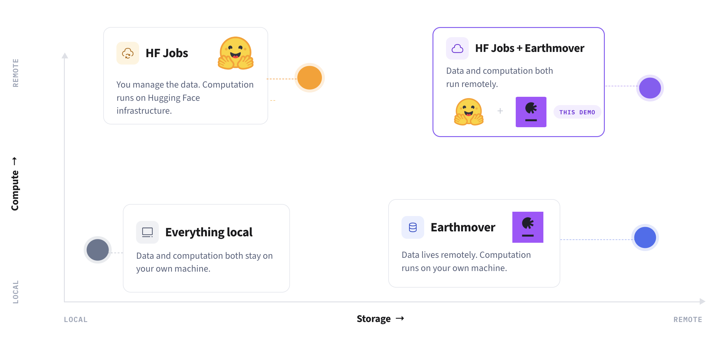
This blog walks you through running weather forecasting models available on Hugging Face using data from Earthmover, so you can spend less time on infrastructure and more time on the science and the forecasting. Earthmover’s data platform takes care of the last two frictions, storage and bandwidth, while for compute, we show how to run the same forecast using Hugging Face jobs in Running the model using Hugging Face jobs.

We will start with a demo and a tutorial, but you can read more about what Earthmover is and what is available for AI for climate on Hugging Face in the sections Earthmover: the Science Data Cloud and What’s next on AI for climate at Hugging Face?.

Running weather forecasting models yourself on our demo space

AI weather forecasting models: how do they work?

AI weather forecasting models are neural networks trained to predict the future state of the atmosphere, the same way LLMs are trained to predict the next word. The difference is what’s being predicted: it is not the next token in a sentence, but the next snapshot of the atmosphere: a 3D grid of temperature, wind, humidity, and other variables at each specific longitude/latitude grid point on Earth (most models use a 0.25° grid), at a given moment.

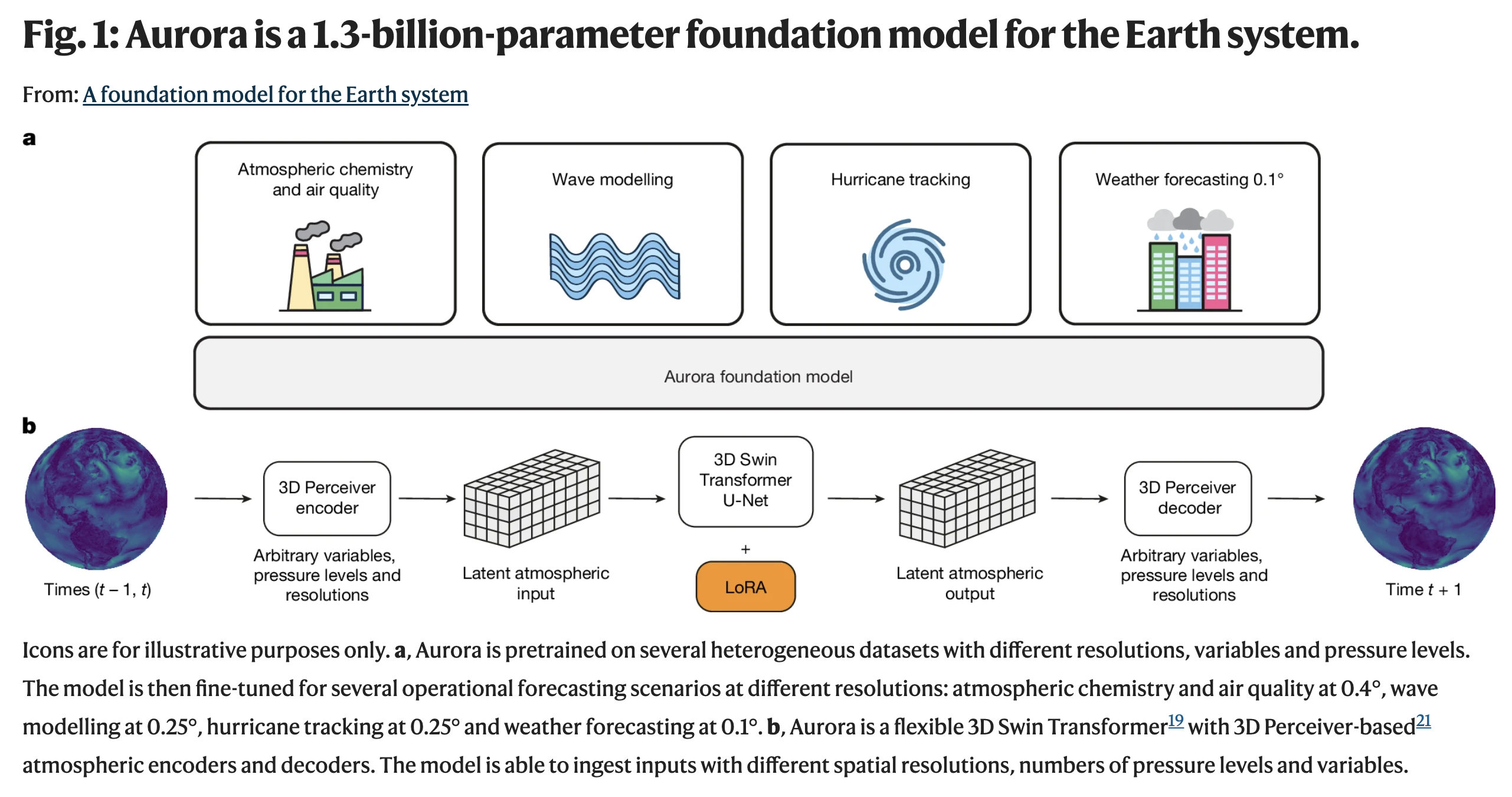
To forecast further out, the model feeds its own output back in as the next input and runs again. It uses the same autoregressive idea as LLMs, generating token by token, except each step here is a full global atmospheric state rather than a word. Under the hood, most of these models (Aurora, AIFS, FourCastNet) use familiar deep learning building blocks (neurons, activation functions and attention layers) just adapted to grids instead of text.

Demo space to run a few models yourself

We have built a demo space that shows how to get initialization data from Earthmover, run a few AI weather models available on the Hub, and compare the results against ERA5. You can run any of the available models on any of the available initialization data directly from the space, and retrieve the resulting forecast from the storage bucket. If you’re interested in the performance, you can see how long each step of the forecast takes (from loading the initial conditions to plotting the forecast): end-to-end, you can get a 24h forecast in under ~30s.

You can run the forecasts below:

Tutorial: running an AI weather forecasting model locally with data from the Earthmover Marketplace

Our goal is to make it easier for the climate community to run such models on their own. So, we provide below an easy-to-follow tutorial on how to run a forecast locally using free data from the Earthmover Marketplace. We’ll walk through a 4-step (24-hour) forecast with Aurora, Microsoft’s atmospheric foundation model, initialized from ERA5 data on Earthmover Marketplace and compared against ERA5. Aurora’s weights are published on the Hub under an MIT license, so you can run, fine-tune, and build on them. We use the aurora-0.25-pretrained checkpoint, which operates on 0.25° ERA5-style inputs and predicts one 6-hour step per forward pass.

Below, we walk through the main elements of the code. You can also find and run the code in this Google colab. If you’d rather skip ahead, the demo space code is available to look at directly.

Before you start: you’ll need a free Hugging Face account (sign up here) to pull Aurora’s weights. You will also need a free Earthmover account (sign up here).

No GPU is required, the forecast takes 2–3 minutes per step, on a CPU and a few seconds on a GPU. Note that MPS is not supported by Aurora.

Fetching the initialization data

Earthmover provides a Python client for reading data directly from your notebook. First, install the required packages and log in with your Earthmover account:

! pip install arraylake xarray microsoft-aurora huggingface_hub matplotlib pcodec cartopy
! arraylake auth login
! hf auth login

Connect to the client:

from arraylake import Client

arraylake_client = Client()
era5_repo = arraylake_client.get_repo("earthmover-public/era5") # requires pcodec
rsession = era5_repo.readonly_session("main")

Note that if you’re having trouble logging in, you can create an ARRAYLAKE_TOKEN instead (how to create a token) and use arraylake_client = Client(token=ARRAYLAKE_TOKEN).

Fetch the initial conditions required to run Aurora:

import xarray as xr

# initial conditions: selected timestamp + previous 6 hours
TIMESTAMPS = ["2026-03-12T18:00:00", "2026-03-13T00:00:00"]

# fetch surface-level fields
era5_single_level = xr.open_zarr(rsession.store, group="single/spatial", chunks=None)
initial_conditions_single_regular_grid = era5_single_level.sel(valid_time=TIMESTAMPS)[
    ["u10", "v10", "d2m", "t2m", "msl", "skt", "sp", "tcw", "stl1", "stl2", "swvl1", "swvl2"]
]

# fetch pressure-level fields
era5_pressure_levels = xr.open_zarr(rsession.store, group="pressure/spatial", chunks=None)
initial_conditions_pressure_regular_grid = era5_pressure_levels.sel(valid_time=TIMESTAMPS)

Aurora’s static variable slt (soil type) isn’t part of the ERA5 archive, and static variables need to match exactly what Aurora was trained on, so all static variables are downloaded from the Hugging Face Hub instead:

import pickle
from huggingface_hub import hf_hub_download

static_path = hf_hub_download(repo_id="microsoft/aurora", filename="aurora-0.25-static.pickle")
with open(static_path, "rb") as f:
    static_vars = pickle.load(f)  # {"lsm": ndarray, "z": ndarray, "slt": ndarray}

Running Aurora

Aurora expects a Batch object with surface variables, static variables, atmospheric variables, and metadata. Build the input batch:

import datetime
import torch
import numpy as np
from aurora import Batch, Metadata

def _tensor(x):
    return torch.from_numpy(np.ascontiguousarray(x, dtype=np.float32))[None]

surf_names = {"2t": "t2m", "10u": "u10", "10v": "v10", "msl": "msl"}
atmos_names = ["t", "u", "v", "q", "z"]

batch = Batch(
    surf_vars={k: _tensor(initial_conditions_single_regular_grid[v].values) for k, v in surf_names.items()},
    static_vars={k: _tensor(v)[0] for k, v in static_vars.items()},
    atmos_vars={k: _tensor(initial_conditions_pressure_regular_grid[k].values) for k in atmos_names},
    metadata=Metadata(
        lat=torch.from_numpy(era5_single_level.latitude.values.astype("f4")),
        lon=torch.from_numpy(era5_single_level.longitude.values.astype("f4")),
        time=(datetime.datetime.fromisoformat(TIMESTAMPS[-1]),),
        atmos_levels=tuple(era5_pressure_levels.pressure_level.values.tolist()),
    ),
)

Load the pretrained model and run 4 steps (a 24h forecast):

from aurora import Aurora, rollout

model = Aurora(use_lora=False)
model.load_checkpoint("microsoft/aurora", "aurora-0.25-pretrained.ckpt")
model.eval()

device = "cuda" if torch.cuda.is_available() else "cpu"
model = model.to(device)

# Aurora predicts one 6-hour step per forward pass. rollout() applies the model autoregressively
STEPS = 4  # 4 x 6h = 24h forecast
with torch.inference_mode():
    predictions = [pred.to("cpu") for pred in rollout(model, batch, steps=STEPS)]

Reassemble forecasts as xr.Dataset:

# assemble as xr.Dataset with metadata as coordinates
import pandas as pd
dims = ["init_time","step","latitude", "longitude"] # order important
meta = predictions[0].metadata
predictions_ds = xr.concat([xr.Dataset(data_vars={v: (dims, predictions[i].surf_vars[v].numpy()) for v in predictions[0].surf_vars}) for i in range(STEPS)], "step")
predictions_ds = predictions_ds.assign_coords(longitude=meta.lon, latitude=meta.lat, init_time=[meta.time[0]], step=[pd.Timedelta(hours=6)*i for i in range(STEPS)])
predictions_ds = predictions_ds.assign_coords(valid_time=predictions_ds.init_time + predictions_ds.step)
predictions_ds = predictions_ds.squeeze().swap_dims({"step":"valid_time"})

import io
import numpy as np
import pandas as pd
import matplotlib.pyplot as plt
import matplotlib as mpl
import imageio.v3 as iio
import cartopy.crs as ccrs

FRAMES_PER_STEP = 12   # rotation frames held per forecast step
N_TURNS = 1            # full rotations across the whole gif
FIGSIZE = (7, 6)
DPI = 120
CMAP = "RdYlBu_r"


def valid_time_label(valid_time):
    """'YYYY-MM-DD HH:MM UTC' for one forecast valid_time."""
    return pd.Timestamp(valid_time).strftime("%Y-%m-%d %H:%M UTC")


def render_frame(data, label, lon, vmin, vmax, norm):
    """One rotated globe frame - RGB array, fixed canvas size for GIF stability."""
    fig = plt.figure(figsize=FIGSIZE, dpi=DPI)
    ax = fig.add_axes(
        [0.03, 0.08, 0.72, 0.84],
        projection=ccrs.Orthographic(central_longitude=lon, central_latitude=20),
    )
    ax.set_global()
    ax.coastlines()
    data.plot(
        ax=ax, transform=ccrs.PlateCarree(),
        vmin=vmin, vmax=vmax, cmap=CMAP, add_colorbar=False, add_labels=False,
    )
    ax.set_title(f"Aurora forecast — 2m temperature\nValid time: {label}", fontsize=10)

    cax = fig.add_axes([0.80, 0.15, 0.03, 0.7])
    fig.colorbar(mpl.cm.ScalarMappable(norm=norm, cmap=CMAP), cax=cax,
                 label="2m temperature [°C]")

    buf = io.BytesIO()
    fig.savefig(buf, format="png")
    plt.close(fig)
    buf.seek(0)
    return iio.imread(buf)


temp = predictions_ds["2t"] - 273.15  # °C, dims: (valid_time, latitude, longitude)

n_steps = temp.valid_time.size
total_frames = n_steps * FRAMES_PER_STEP
vmin, vmax = np.nanpercentile(temp.values, [2, 98])
norm = mpl.colors.Normalize(vmin=vmin, vmax=vmax)

frames = []
for i in range(n_steps):
    data = temp.isel(valid_time=i)
    label = valid_time_label(temp.valid_time.values[i])

    for j in range(FRAMES_PER_STEP):
        frame_idx = i * FRAMES_PER_STEP + j
        lon = (frame_idx * 360 * N_TURNS / total_frames) % 360
        frames.append(render_frame(data, label, lon, vmin, vmax, norm))

iio.imwrite("aurora_forecast_rotating.gif", frames, duration=220, loop=0)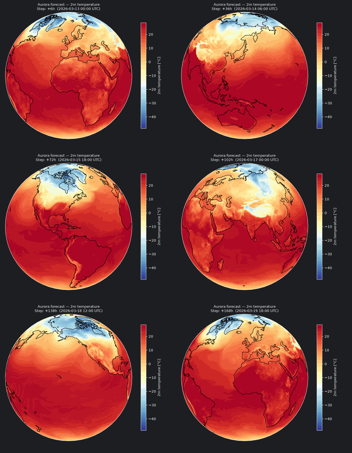

Comparing Aurora’s forecast with ERA5

Aurora’s forecast is only useful if you can tell how good it is. Since the model was initialized from ERA5, the natural way to check it is to compare the forecast against ERA5’s own state at the same valid time, and compute the RMSE between the two.

Calculate the difference to see where the forecast differs from ERA5:

bias = predictions_ds["2t"] - era5_single_level["t2m"] # automatic broadcasting: https://docs.xarray.dev/en/latest/user-guide/computation.html#broadcasting-by-dimension-name
weights = np.cos(np.deg2rad(bias.latitude))
global_rmse = (bias ** 2).weighted(weights).mean(["longitude", "latitude"]) ** 0.5

import io
import pandas as pd
import xarray as xr
import matplotlib.pyplot as plt
import matplotlib as mpl
import imageio.v3 as iio
import cartopy.crs as ccrs
from arraylake import Client

FRAMES_PER_STEP = 4    # rotation frames held per forecast step
N_TURNS = 2            # full rotations across the whole gif
FIGSIZE = (7, 6)
DPI = 120
CMAP = "RdBu_r"
OUTPUT_PATH = "aurora_error_rotating.gif"


def load_era5_single_level():
    client = Client()
    repo = client.get_repo("earthmover-public/era5")
    session = repo.readonly_session("main")
    return xr.open_zarr(session.store, group="single/spatial", chunks=None)


def compute_bias(predictions_ds, era5_single_level):
    """Forecast − ERA5, matched to the forecast's valid times and regridded
    onto the forecast's lat/lon grid. Returns an in-memory (computed) DataArray."""
    init_time = predictions_ds["init_time"].values[0]
    valid_times = pd.Timestamp(init_time) + pd.to_timedelta(predictions_ds["step"].values)

    era5_matched = (
        era5_single_level["t2m"]
        .sel(valid_time=valid_times, method="nearest")
        .rename({"valid_time": "step", "latitude": "lat", "longitude": "lon"})
        .assign_coords(step=predictions_ds["step"].values)
    )

    forecast = predictions_ds["2t"].isel(init_time=0)
    era5_matched = era5_matched.reindex_like(forecast, method="nearest", tolerance=0.3)

    bias = (forecast - era5_matched).compute()
    return bias, init_time


def compute_global_rmse(bias):
    weights = np.cos(np.deg2rad(bias.lat))
    return ((bias ** 2).weighted(weights).mean(["lat", "lon"]) ** 0.5).compute()


def step_label(init_time, step_timedelta):
    """'+Nh  (YYYY-MM-DD HH:MM UTC)' for one forecast step."""
    hours = int(step_timedelta / np.timedelta64(1, "h"))
    valid_dt = pd.Timestamp(init_time) + pd.Timedelta(step_timedelta)
    return f"+{hours}h  ({valid_dt.strftime('%Y-%m-%d %H:%M')} UTC)"


def render_frame(data, label, rmse, lon, vmin, vmax, norm):
    """One rotated globe frame - RGB array, fixed canvas size for GIF stability."""
    fig = plt.figure(figsize=FIGSIZE, dpi=DPI)
    ax = fig.add_axes(
        [0.03, 0.08, 0.72, 0.84],
        projection=ccrs.Orthographic(central_longitude=lon, central_latitude=20),
    )
    ax.set_global()
    ax.coastlines()
    data.plot(
        ax=ax, transform=ccrs.PlateCarree(),
        vmin=vmin, vmax=vmax, cmap=CMAP, add_colorbar=False, add_labels=False,
    )
    ax.set_title(
        f"Aurora error - ERA5 — 2m temperature\nStep: {label}  ·  RMSE = {rmse:.2f}K",
        fontsize=10,
    )

    cax = fig.add_axes([0.80, 0.15, 0.03, 0.7])
    fig.colorbar(mpl.cm.ScalarMappable(norm=norm, cmap=CMAP), cax=cax,
                 label="2m temperature bias [K]")

    buf = io.BytesIO()
    fig.savefig(buf, format="png")
    plt.close(fig)
    buf.seek(0)
    return iio.imread(buf)


def build_frames(bias, global_rmse, init_time):
    n_steps = bias.step.size
    total_frames = n_steps * FRAMES_PER_STEP

    limit = float(np.nanmax(np.abs(np.nanpercentile(bias.values, [2, 98]))))
    vmin, vmax = -limit, limit
    norm = mpl.colors.Normalize(vmin=vmin, vmax=vmax)

    frames = []
    for i in range(n_steps):
        data = bias.isel(step=i)
        label = step_label(init_time, bias.step.values[i])
        rmse = float(global_rmse.isel(step=i).values)

        for j in range(FRAMES_PER_STEP):
            frame_idx = i * FRAMES_PER_STEP + j
            lon = (frame_idx * 360 * N_TURNS / total_frames) % 360
            frames.append(render_frame(data, label, rmse, lon, vmin, vmax, norm))

    assert len(set(f.shape for f in frames)) == 1, "frame size mismatch"
    return frames


era5_single_level = load_era5_single_level()
bias, init_time = compute_bias(predictions_ds, era5_single_level)
global_rmse = compute_global_rmse(bias)

frames = build_frames(bias, global_rmse, init_time)
iio.imwrite(OUTPUT_PATH, frames, duration=220, loop=0)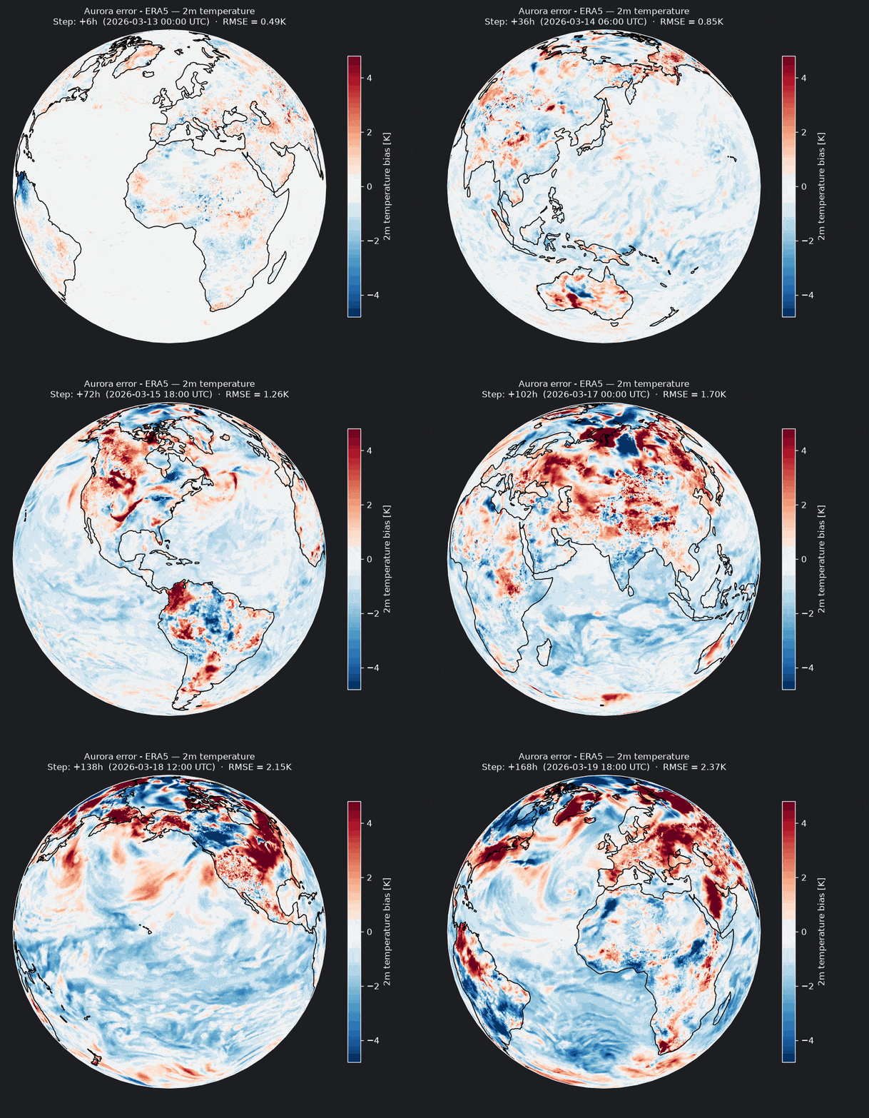

Running the model using Hugging Face jobs

If you don’t have the right hardware locally, Hugging Face Jobs let you run inference on Hugging Face’s infrastructure, billed per minute only while the job is running. There is no cost during building, or if a job fails. Results can be pushed to a storage bucket you choose, private or public. We use NVIDIA A100 Large ($2.50/hour).

To run the forecast with Hugging Face job, you will need an HF_TOKEN (how to create a token) with a permission to start and manage jobs. You will also need an ARRAYLAKE_TOKEN (see above).

Save the code below in a file named run_aurora_forecast.py and replace your-hf-username with your HF username.

# /// script
# dependencies = [
#   "arraylake",
#   "xarray",
#   "microsoft-aurora",
#   "huggingface_hub",
#   "pcodec",
# ]
# ///

from arraylake import Client
import xarray as xr
import pickle
import datetime
import torch
from aurora import Batch, Metadata, Aurora, rollout
import pandas as pd
import numpy as np
from huggingface_hub import login, hf_hub_download
import os

login()

STEPS = 28  # 28 x 6h = 7 days forecast

arraylake_client = Client(token=os.environ["ARRAYLAKE_TOKEN"])
era5_repo = arraylake_client.get_repo("earthmover-public/era5")
rsession = era5_repo.readonly_session("main")

# initial conditions: selected timestamp + previous 6 hours
TIMESTAMPS = ["2026-03-12T18:00:00", "2026-03-13T00:00:00"]

# fetch surface-level fields
era5_single_level = xr.open_zarr(rsession.store, group="single/spatial", chunks=None)
initial_conditions_single_regular_grid = era5_single_level.sel(valid_time=TIMESTAMPS)[
    ["u10", "v10", "d2m", "t2m", "msl", "skt", "sp", "tcw", "stl1", "stl2", "swvl1", "swvl2"]
]

# fetch pressure-level fields
era5_pressure_levels = xr.open_zarr(rsession.store, group="pressure/spatial", chunks=None)
initial_conditions_pressure_regular_grid = era5_pressure_levels.sel(valid_time=TIMESTAMPS)


static_path = hf_hub_download(repo_id="microsoft/aurora", filename="aurora-0.25-static.pickle")
with open(static_path, "rb") as f:
    static_vars = pickle.load(f)  # {"lsm": ndarray, "z": ndarray, "slt": ndarray}

def _tensor(x):
    return torch.from_numpy(np.ascontiguousarray(x, dtype=np.float32))[None]

surf_names = {"2t": "t2m", "10u": "u10", "10v": "v10", "msl": "msl"}
atmos_names = ["t", "u", "v", "q", "z"]

batch = Batch(
    surf_vars={k: _tensor(initial_conditions_single_regular_grid[v].values) for k, v in surf_names.items()},
    static_vars={k: _tensor(v)[0] for k, v in static_vars.items()},
    atmos_vars={k: _tensor(initial_conditions_pressure_regular_grid[k].values) for k in atmos_names},
    metadata=Metadata(
        lat=torch.from_numpy(era5_single_level.latitude.values.astype("f4")),
        lon=torch.from_numpy(era5_single_level.longitude.values.astype("f4")),
        time=(datetime.datetime.fromisoformat(TIMESTAMPS[-1]),),
        atmos_levels=tuple(era5_pressure_levels.pressure_level.values.tolist()),
    ),
)

model = Aurora(use_lora=False)
model.load_checkpoint("microsoft/aurora", "aurora-0.25-pretrained.ckpt")
model.eval()

device = "cuda" if torch.cuda.is_available() else "cpu"
model = model.to(device)

# Aurora predicts one 6-hour step per forward pass. rollout() applies the model autoregressively
with torch.inference_mode():
    predictions = []
    for pred in rollout(model, batch, steps=STEPS):
        predictions.append(pred.to("cpu"))
        torch.cuda.empty_cache()

# assemble as xr.Dataset with metadata as coordinates
dims = ["init_time","step","latitude", "longitude"] # order important
meta = predictions[0].metadata
predictions_ds = xr.concat([xr.Dataset(data_vars={v: (dims, predictions[i].surf_vars[v].numpy()) for v in predictions[0].surf_vars}) for i in range(STEPS)], "step")
predictions_ds = predictions_ds.assign_coords(longitude=meta.lon, latitude=meta.lat, init_time=[meta.time[0]], step=[pd.Timedelta(hours=6)*i for i in range(STEPS)])
predictions_ds = predictions_ds.assign_coords(valid_time=predictions_ds.init_time + predictions_ds.step)
predictions_ds = predictions_ds.squeeze().swap_dims({"step":"valid_time"})

# save forecast to bucket
predictions_ds.to_zarr(f"hf://buckets/your-hf-username/aurora-forecasts/forecast_{TIMESTAMPS[-1]}.zarr")

Create a bucket named your-hf-username/aurora-forecasts.

Run the following command:

hf jobs uv run --flavor a100-large --secrets HF_TOKEN --secrets ARRAYLAKE_TOKEN --with pcodec run_aurora_forecast.py

Earthmover: the Science Data Cloud

Why is Earthmover efficient for scientific data?

Earthmover is a data platform for weather, climate, and earth-observation data. It is built on two open-source technologies that make it fast to fetch the data you need, rather than downloading whole files:

• Zarr, a data format for storing large, multi-dimensional arrays as many small, independently readable chunks rather than one large file. It makes it possible to fetch just the necessary variables, levels, or timesteps.
• Icechunk, which adds a transactional storage layer on top of Zarr: version control, safe concurrent writes, and consistent snapshots of your data, similar to what Git gives you for code.

This is why the Earthmover Marketplace is a good fit for fetching initial conditions: data can be streamed at gigabyte-per-second speeds even though it is not stored locally. This removes the bandwidth bottleneck: instead of downloading a whole file to get the few variables you need, you fetch exactly those bytes, directly from the cloud, at high throughput.

Earthmover allows teams to store and manage their own private datasets but also hosts a Data Marketplace containing over 60 PB of analysis-ready weather, climate, and earth-observation data. The marketplace enables organizations to easily exchange data in the cloud without having to pre-download huge archives.

Initializing data to run an AI weather forecast

To run and backtest an AI forecast, you need data to initialize the model with, and data to check its predictions against. But there’s no single global “ground truth” for the atmosphere: weather stations, satellites, and balloons each observe only a small part of the global data. The closest to “ground truth” is an analysis (or a reanalysis for historic data): a dataset that assimilates observations using a physics model. That’s what we use for both initializing and backtesting forecast models.

Earthmover’s Marketplace hosts two open datasets you can use for this:

• ECMWF ERA5: a reanalysis dataset going back hourly to 1940. This is what we use both to initialize Aurora and to evaluate its forecast afterward. Earthmover’s free plan lags 3–6 months behind real time; a paid plan brings you up to 6 days ago, which is what we use in our demo.
• ECMWF IFS: the initial conditions of ECMWF’s operational physics-based forecast, as a rolling archive covering the last 15 days.

Once your AI weather forecast has been generated, you can store it back on Earthmover’s Arraylake platform, in the same Icechunk format, on a storage bucket on most major cloud providers: Hugging Face bucket, which offers a 100GB free tier, AWS S3, Cloudflare R2 (including a 10GB community free tier managed by Earthmover), or GCS.

What’s next on AI for climate at Hugging Face?

Open weather models on the Hub

Many open-source weather forecasting model weights are available on the Hugging Face Hub, including:

• ECMWF AIFS
• Microsoft Aurora
• NVIDIA Atlas
• NVIDIA FourCastNet
• Prithvi

Some of these models need specific hardware to run efficiently. AIFS, for instance, depends on flash attention, which only works on certain GPU architectures. If you don’t have access to this hardware, you can read our previous blog post ECMWF’s AI forecasting model is open source, where we explain how to run AIFS Single 2.0 on other GPUs or using Hugging Face jobs. We’re also in the process of integrating these models into the transformers library, so they can be run with fewer dependencies and fine-tuned using transformers.Trainer.

What’s next

Hopefully, this blog post showed how easily you can run AI weather models hosted on Hugging Face using data from the Earthmover Marketplace.

What we will do next depends on what the climate community needs, and therefore on the feedback we get on this blog post and the demo space. In general, we’d love to bring more open models in, including smaller models and models fine-tuned by the community. We’re currently working on integrating models like Google’s WeatherNext 2 into transformers, which will make inference way easier (less code and fewer dependencies to fight with) and open the door to fine-tuning right on Hugging Face Jobs.

Some points for which we’d love to hear from you:

• What do you like about the demo?
• What’s missing?
• What do you use it for?

Please reach out to us via the blog post comments, the space discussions or by email.